genomeNLP: Case study of DNA

4. Setting up a biological dataset

Understanding of the data and experimental design is a necessary first step to analysis. In our case study, we perform a simple two case classification, where the dataset consists of a corpora of biological sequence data belonging to two categories. Genomic sequence associated with promoters and non-promoter regions are available. In the context of biology, promoters are important modulators of gene expression, and most are relatively short as well as information rich. Motif prediction is an active, on-going area of research in biology, since many of these signals are weak and difficult to detect, as well as varying in frequency and distribution across different species. Therefore, our aim is to classify sequences into promoter and non-promoter sequence categories.

Note

A more detailed description of the data is available here.

Our data is available in the form of fasta files. fasta files are a common format for storing biological sequence data. They typically contain headers that provide information about the sequence, followed by the sequence itself. They can also store other nucleic acid data, as well as protein. The fasta format contains headers with a leading >. Lines without > contain biological sequence data and can be newline separated. In our simple example, the full set of characters are the DNA nucleotides adenine A, thymine T, cytosine C and guanine G. These are the building blocks of the genetic code.

The files can be downloaded here for non promoter sequences and promoter sequences.

# create the directory structure
cd ~
mkdir -p data src results
cd data
curl -L -O "https://raw.githubusercontent.com/khanhlee/bert-promoter/main/data/non_promoter.fasta"
curl -L -O "https://raw.githubusercontent.com/khanhlee/bert-promoter/main/data/promoter.fasta"
gzip non_promoter.fasta
gzip promoter.fasta

HEADER:   >PCK12019 FORWARD 639002 STRONG
SEQUENCE: TAGATGTCCTTGATTAACACCAAAAT
HEADER:   >ECK12066 REVERSE 3204175 STRONG
SEQUENCE: AAAGAAAATAATTAATTTTACAGCTG

Note

In real world data, other characters are available which refer to multiple possible nucleotides, for example ``W`` indicates either an ``A`` or a ``T``. RNA includes the character ``U``, and proteins include additional letters of the alphabet.

Tokenisation in genomics involves segmenting biological sequences into smaller units, called tokens (or k-mers in biology) for further processing. In the context of genomics, tokens can represent individual nucleotides, k-mers, codons, or other biologically meaningful segments. Just as in conventional NLP, tokenisation is required to facilitate most downstream operations.

Here, we provide gzipped fasta file(s) as input. While conventional biological tokenisation splits a sequence into arbitrary-length segments, empirical tokenisation derives the resulting tokens directly from the corpus, with vocabulary size as the only user-defined parameter. Data is then split into training, testing and/or validation partitions as desired by the user and automatically reformatted for input into the deep learning pipeline.

Note

We provide the conventional k-merisation method as well as an option for users. In our pipeline specifically, the empirical tokenisation and data object creation is split into two steps, while k-merisation combines both in one operation. This is due to the empirical tokenisation process having to “learn” tokens from the data.

# Empirical tokenisation pathway
cd ~/src
tokenise_bio \
  -i ../data/promoter.fasta.gz \
     ../data/non_promoter.fasta.gz \
  -t ../data/tokens.json
# -i INFILE_PATHS path to files with biological seqs split by line
# -t TOKENISER_PATH path to tokeniser.json file to save or load data

This generates a json file with tokens and their respective weights or IDs. You should see some output like this.

[00:00:00] Pre-processing sequences
[00:00:00] Suffix array seeds
[00:00:14] EM training
Sample input sequence: AACCGGTT
Sample tokenised: [156, 2304]
Token: : k-mer map: 156  : : AA
Token: : k-mer map: 2304 : : CCGGTT

5. Format a dataset for input into genomeNLP

In this section, we reformat the data to meet the requirements of our pipeline which takes specifically structured inputs. This intermediate data structure serves as the foundation for downstream analyses and facilitates seamless integration with the pipeline. Our pipeline contains a method that performs this automatically, generating a reformatted dataset with the desired structure.

Note

The data format is identical to that used by the HuggingFace ``datasets`` and ``transformers`` libraries.

# Empirical tokenisation pathway
create_dataset_bio \
  ../data/promoter.fasta.gz \
  ../data/non_promoter.fasta.gz \
  ../data/tokens.json \
  -o ../data/
# -o OUTFILE_DIR write dataset to directory as
#   [ csv \| json \| parquet \| dir/ ] (DEFAULT:"hf_out/")
# default datasets split: train 90%, test 5% and validation set 5%

The output is a reformatted dataset containing the same information. Properties required for a typical machine learning pipeline are added, including labels, customisable data splits and token identifiers.

DATASET AFTER SPLIT:
DatasetDict ({
  train: Dataset ({
  features: ['idx', 'feature', 'labels', 'input_ids', 'token_type_ids', 'attention_mask’],
  num_rows: 12175 })
  test: Dataset ({
  features: ['idx', 'feature', 'labels', 'input_ids', 'token_type_ids', 'attention_mask’],
  num_rows: 677 })
  valid: Dataset ({
  features: ['idx', 'feature', 'labels', 'input_ids', 'token_type_ids', 'attention_mask’],
  num_rows: 676 })
})

Note

The column ``token_type_ids`` is not actually needed in this specific case study, but it is safely ignored in such cases.

SAMPLE TOKEN MAPPING FOR FIRST 5 TOKENS IN SEQ:
TOKEN ID: 858  | TOKEN: TCA
TOKEN ID: 2579 | TOKEN: GCATCAC
TOKEN ID: 111  | TOKEN: TATT
TOKEN ID: 99   | TOKEN: CAGG
TOKEN ID: 777  | TOKEN: AGGCT

6. Preparing a hyperparameter sweep

In machine learning, achieving optimal model performance often requires finding the right combination of hyperparameters (assuming the input data is viable). Hyperparameters vary depending on the specific algorithm and framework being used, but commonly include learning rate, dropout rate, batch size, number of layers and optimiser choice. These parameters heavily influence the learning process and subsequent performance of the model.

For this reason, hyperparameter sweeps are normally carried out to systematically test combinations of hyperparameters, with the end goal of identifying the configuration that produces the best model performance. Usually, sweeps are carried out on a small partition of the data only to maximise efficiency of compute resources, but it is not uncommon to perform sweeps on entire datasets. Various strategies, such as grid search, random search, or bayesian optimisation, can be employed during a hyperparameter sweep to sample parameter values. Additional strategies such as early stopping can also be used.

To streamline the hyperparameter optimization process, we use the wandb (Weights & Biases) platform which has a user-friendly interface and powerful tools for tracking experiments and visualising results.

First, sign up for a wandb account at: https://wandb.ai/site and login by pasting your API key.

wandb login
wandb: Paste an API key from your profile, and hit enter and hit enter or press ctrl+c to quit:

Now, we use the sweep tool to perform hyperparameter sweep. Search strategy, parameters and search space are passed in as a json file. An example is below. If no sweep configuration is provided, default configuration will apply.

Default hyperparameter sweep settings if none are provided. You can copy this file and edit it for your own use if needed.

{
    "name": "random",
    "method": "random",
    "metric": {
        "name": "eval/f1",
        "goal": "maximize"
        },
    "parameters": {
        "epochs": {
            "values": [1, 2, 3, 4, 5]
            },
        "dropout": {
          "values": [0.15, 0.2, 0.25, 0.3, 0.4]
        },
        "batch_size": {
            "values": [8, 16, 32, 64]
            },
        "learning_rate": {
            "distribution": "log_uniform_values",
            "min": 1e-5,
            "max": 1e-1
        },
        "weight_decay": {
            "values": [0.0, 0.1, 0.2, 0.3, 0.4, 0.5]
        },
        "decay": {
            "values": [1e-5, 1e-6, 1e-7]
        },
        "momentum": {
            "values": [0.8, 0.9, 0.95]
        }
    },
    "early_terminate": {
        "type": "hyperband",
        "s": 2,
        "eta": 3,
        "max_iter": 27
    }
}

sweep \
  ../data/train.parquet \
  parquet \
  ../data/tokens.json \
  -t ../data/test.parquet \
  -v ../data/valid.parquet \
  -w ../data/hyperparams.json \   # optional
  -e entity_name \       # <- edit as needed
  -p project_name \      # <- edit as needed
  -l labels \
  -n 3
# -t TEST, path to [ csv \| csv.gz \| json \| parquet ] file
# -v VALID, path to [ csv \| csv.gz \| json \| parquet ] file
# -w HYPERPARAMETER_SWEEP, run a hyperparameter sweep with config from file
# -e ENTITY_NAME, wandb team name (if available).
# -p PROJECT_NAME, wandb project name (if available)
# -l LABEL_NAMES, provide column with label names (DEFAULT: "").
# -n SWEEP_COUNT, run n hyperparameter sweeps

*****Running training*****
Num examples = 12175
Num epochs= 1
Instantaneous batch size per device = 64
Total train batch size per device = 64
Gradient Accumulation steps= 1
Total optimization steps= 191

The output is written to the specified directory, in this case sweep_out and will contain the output of a standard pytorch saved model, including some wandb specific output.

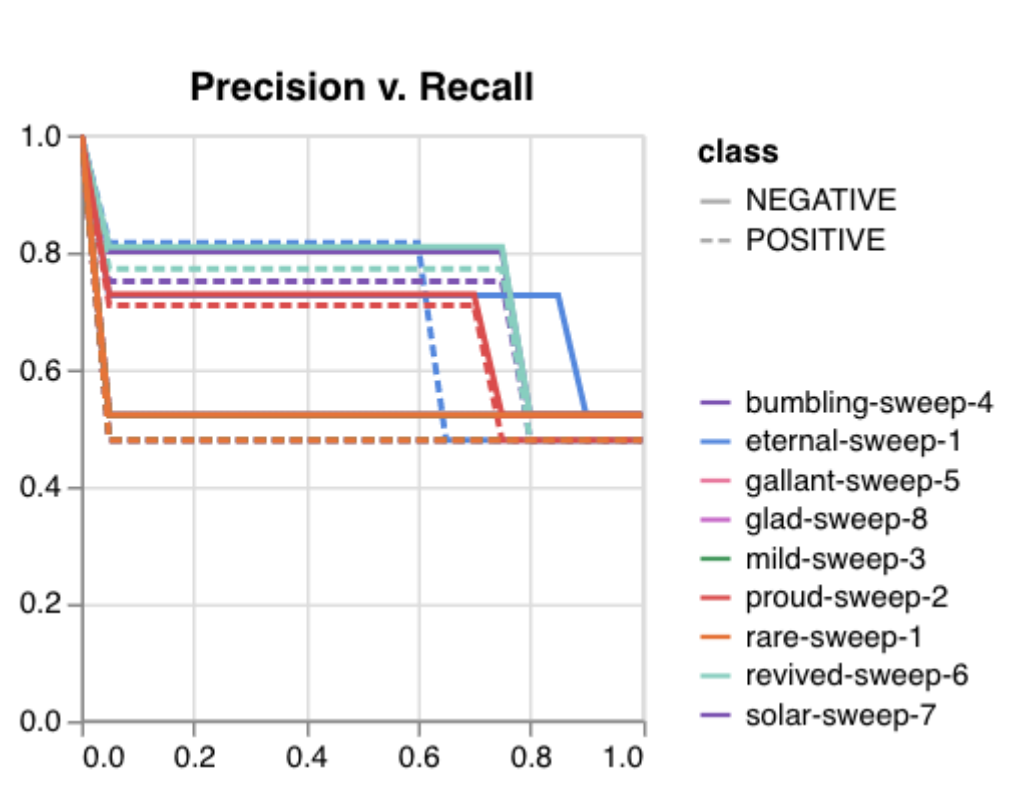
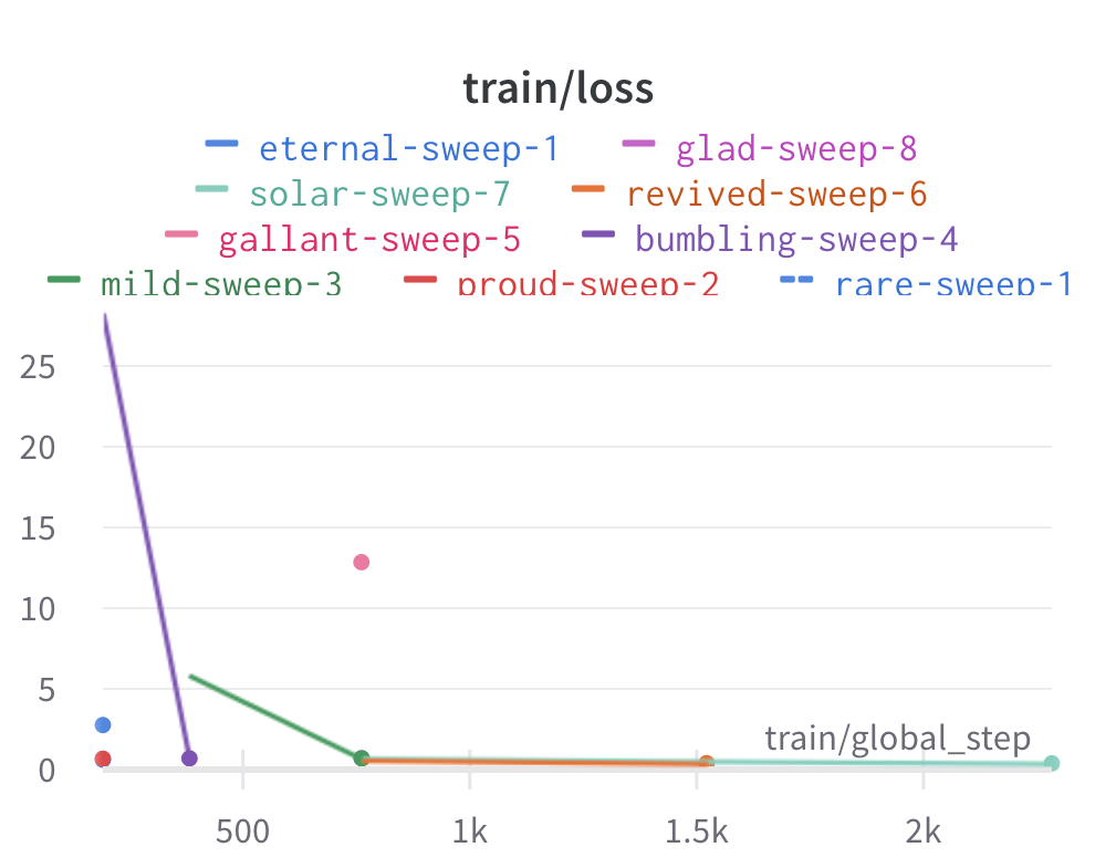
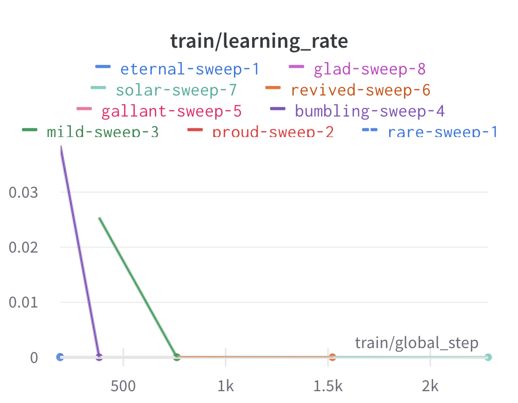
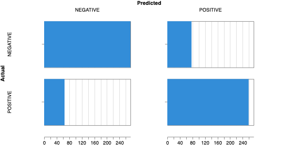
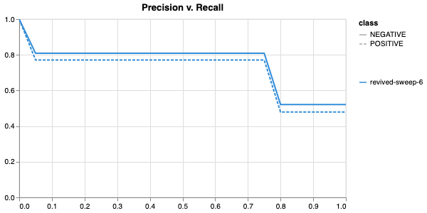
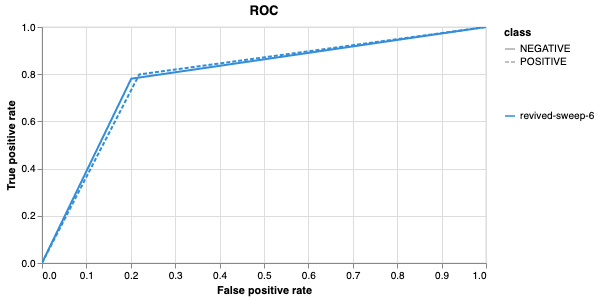
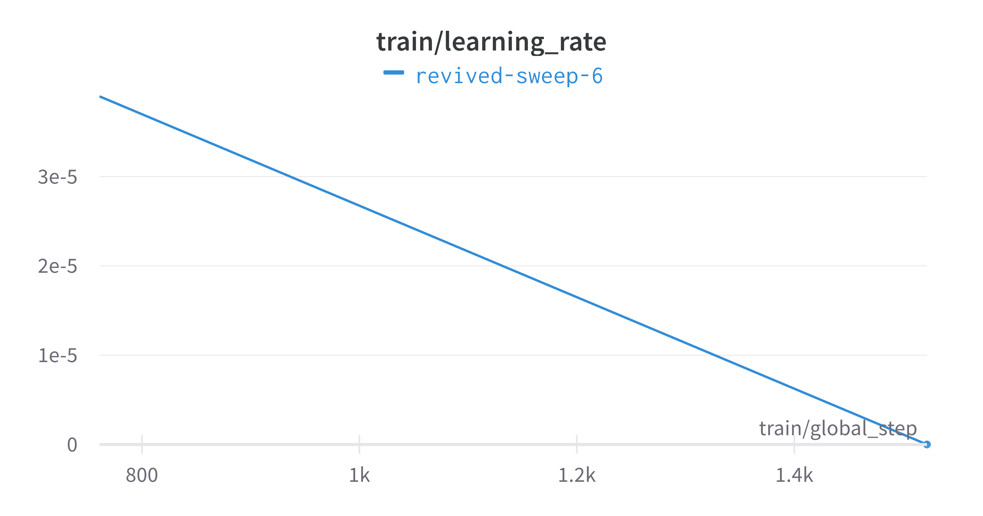
The sweeps gets synced to the wandb dashboard along with various interactive custom charts and tables which we provide as part of our pipeline. A small subset of plots are provided for reference. Interactive versions of these and more plots are available on wandb.

Here is an example of a full wandb generated report:

You may inspect your own generated reports after they complete.

7. Selecting optimal hyperparameters for training

Having completed a sweep, we next identified the best set of parameters for model training. We do this by examining training metrics. These serve as quantitative measures of a model’s performance during training. These metrics provide insights into the model’s accuracy and generalisation capabilities. We explore commonly used training metrics, including accuracy, loss, precision, recall, and f1 score to inform us of a model’s performance

A key event we want to avoid is overfitting. Overfitting occurs when a learning model performs exceptionally well on the training data but fails to generalise to unseen data, making it unfit for use outside of the specific scope of the experiment. This can be detected by observing performance metrics, if the accuracy decreases and later increases an overfit event has occurred. In real world applications, this can lead to adverse events that directly impact us, considering that such models are used in applications such as drug prediction or self-driving cars. Here, we use the f1 score calculated on the testing set as the main metric of interest. We showed that we obtain a best f1 score of 0.79.

Best run revived-sweep-6 with eval/f1=0.7900291349379833
BEST MODEL AND CONFIG FILES SAVED TO: *./sweep_out/model_files*
HYPERPARAMETER SWEEP END

Here is an example of a full wandb generated report for the “best” run.

You may inspect your own generated reports after they complete.

8. With the selected hyperparameters, train the full dataset

In a conventional workflow, the sweep is performed on a small subset of training data. The resulting parameters are then recorded and used in the actual training step on the full dataset. Here, we perform the sweep on the entire dataset, and hence remove the need for further training. If you perform this on your own data and want to use a small subset, you can do so and then pass the recorded hyperparameters with the same input data to the train function of the pipeline. We include an example of this below for completeness, but you can skip this for our specific case study. Note that the input is almost identical to sweep.

train \
  ../data/train.parquet \
  parquet \
  ../data/tokens.json \
  -t ../data/test.parquet \
  -v ../data/valid.parquet \
  --output_dir ../results/train_out \
  -f ../data/hyperparams.json \  # <- you can pass in hyperparameters
  -c entity_name/project_name/run_id \  # <- wandb overrides hyperparameters
  -e entity_name \   # <- edit as needed
  -p project_name    # <- edit as needed
# -t TEST, path to [ csv \| csv.gz \| json \| parquet ] file
# -v VALID, path to [ csv \| csv.gz \| json \| parquet ] file
# -w HYPERPARAMETER_SWEEP, run a hyperparameter sweep with config from file
# -e ENTITY_NAME, wandb team name (if available).
# -p PROJECT_NAME, wandb project name (if available)
# -l LABEL_NAMES, provide column with label names (DEFAULT: "").

Note

Remove the ``-e entity_name`` line if you do not have a group setup in wandb

The contents of hyperparams.json, the file with the best hyperparameters identified by the sweep.

{
  "output_dir": "./sweep_out/random",
  "overwrite_output_dir": false,
  "do_train": false,
  "do_eval": true,
  "do_predict": false,
  "evaluation_strategy": "epoch",
  "prediction_loss_only": false,
  "per_device_train_batch_size": 16,
  "per_device_eval_batch_size": 16,
  "per_gpu_train_batch_size": null,
  "per_gpu_eval_batch_size": null,
  "gradient_accumulation_steps": 1,
  "eval_accumulation_steps": null,
  "eval_delay": 0,
  "learning_rate": 7.796477400405317e-05,
  "weight_decay": 0.5,
  "adam_beta1": 0.9,
  "adam_beta2": 0.999,
  "adam_epsilon": 1e-08,
  "max_grad_norm": 1.0,
  "num_train_epochs": 2,
  "max_steps": -1,
  "lr_scheduler_type": "linear",
  "warmup_ratio": 0.0,
  "warmup_steps": 0,
  "log_level": "passive",
  "log_level_replica": "passive",
  "log_on_each_node": true,
  "logging_dir": "./sweep_out/random/runs/out",
  "logging_strategy": "epoch",
  "logging_first_step": false,
  "logging_steps": 500,
  "logging_nan_inf_filter": true,
  "save_strategy": "epoch",
  "save_steps": 500,
  "save_total_limit": null,
  "save_on_each_node": false,
  "no_cuda": false,
  "use_mps_device": false,
  "seed": 42,
  "data_seed": null,
  "jit_mode_eval": false,
  "use_ipex": false,
  "bf16": false,
  "fp16": false,
  "fp16_opt_level": "O1",
  "half_precision_backend": "auto",
  "bf16_full_eval": false,
  "fp16_full_eval": false,
  "tf32": null,
  "local_rank": -1,
  "xpu_backend": null,
  "tpu_num_cores": null,
  "tpu_metrics_debug": false,
  "debug": [],
  "dataloader_drop_last": false,
  "eval_steps": null,
  "dataloader_num_workers": 0,
  "past_index": -1,
  "run_name": "./sweep_out/random",
  "disable_tqdm": false,
  "remove_unused_columns": false,
  "label_names": null,
  "load_best_model_at_end": true,
  "metric_for_best_model": "loss",
  "greater_is_better": false,
  "ignore_data_skip": false,
  "sharded_ddp": [],
  "fsdp": [],
  "fsdp_min_num_params": 0,
  "fsdp_transformer_layer_cls_to_wrap": null,
  "deepspeed": null,
  "label_smoothing_factor": 0.0,
  "optim": "adamw_hf",
  "adafactor": false,
  "group_by_length": false,
  "length_column_name": "length",
  "report_to": [
    "wandb"
  ],
  "ddp_find_unused_parameters": null,
  "ddp_bucket_cap_mb": null,
  "dataloader_pin_memory": true,
  "skip_memory_metrics": true,
  "use_legacy_prediction_loop": false,
  "push_to_hub": false,
  "resume_from_checkpoint": null,
  "hub_model_id": null,
  "hub_strategy": "every_save",
  "hub_token": "<HUB_TOKEN>",
  "hub_private_repo": false,
  "gradient_checkpointing": false,
  "include_inputs_for_metrics": false,
  "fp16_backend": "auto",
  "push_to_hub_model_id": null,
  "push_to_hub_organization": null,
  "push_to_hub_token": "<PUSH_TO_HUB_TOKEN>",
  "mp_parameters": "",
  "auto_find_batch_size": false,
  "full_determinism": false,
  "torchdynamo": null,
  "ray_scope": "last",
  "ddp_timeout": 1800
}

The output is written to the specified directory, in this case train_out and will contain the output of a standard pytorch saved model, including some wandb specific output.

The trained model gets synced to the wandb dashboard along with various interactive custom charts and tables which we provide as part of our pipeline. A small subset of plots are provided for reference. Interactive versions of these and more plots are available on wandb.

Here is an example of a full wandb generated report:

You may inspect your own generated reports after they complete.

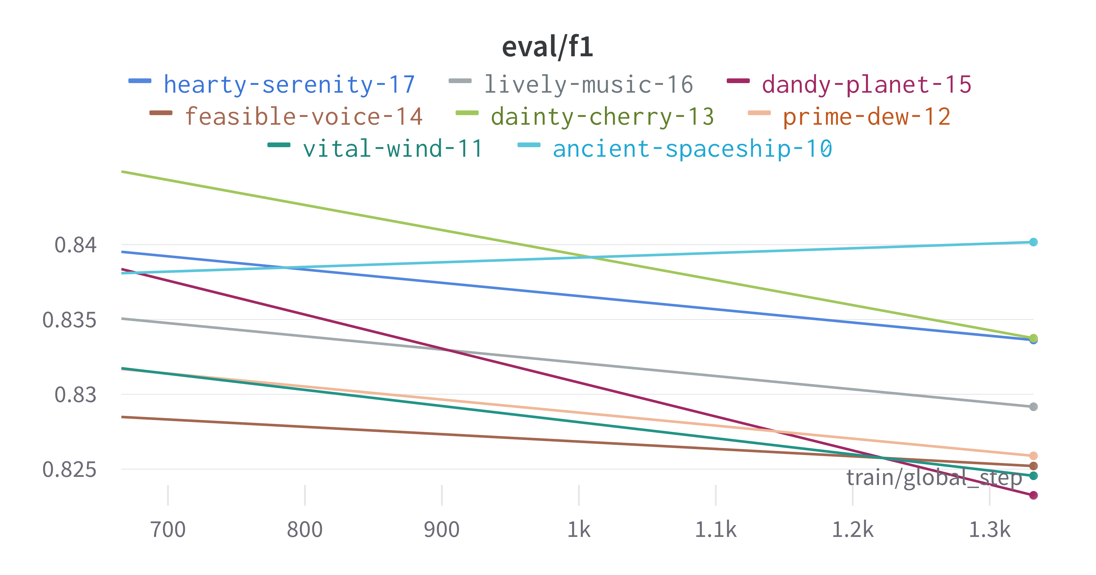
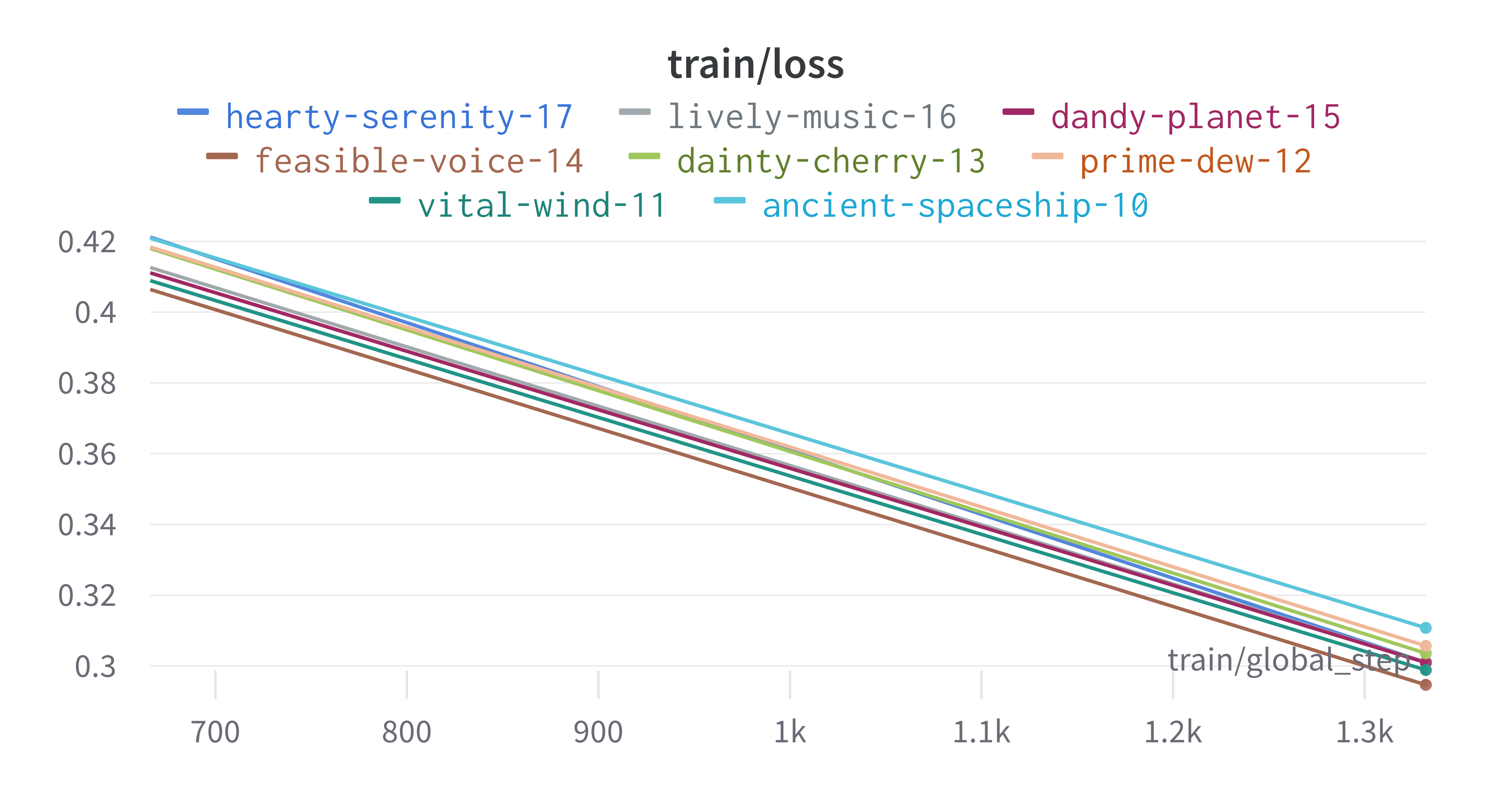
9. Perform cross-validation

Having identified the best set of parameters and trained the model, we next want to conduct a comprehensive review of data stability, and we do this by evaluating model performance across different data slices. This assessment is known as cross-validation. We make use of k-fold cross-validation in which data is divided into k subsets and the model is trained and tested on these individual subsets.

cross_validate \
  ../data/train.parquet parquet \
  -t ../data/test.parquet \
  -v ../data/valid.parquet \
  -e entity_name \              # <- edit as needed
  -p project_name \             # <- edit as needed
  --config_from_run p9do3gzl \  # id OR directory of best performing run
  --output_dir ../results/cv \
  -m ../results/sweep_out \     # <- overridden by --config_from_run
  -l labels \
  -k 8
# --config_from_run WANDB_RUN_ID, *best run id*
# –-output_dir OUTPUT_DIR
# -l label_names
# -k KFOLDS, run n number of kfolds

cross_validate \
  ../data/train.parquet parquet \
  -t ../data/test.parquet \
  -v ../data/valid.parquet \
  -e tyagilab \
  -p foobar \
  -c tyagilab/foobar/kixu82co \
  -o ../results/cv \
  -m ../results/sweep_out \
  -l labels \
  -k 8

Note

If both ``model_path`` and ``config_from_run`` are specified, ``config_from_run`` overrides

Note

Remove the ``-e entity_name`` line if you do not have a group setup in wandb

*****Running training*****
Num examples = 10653
Num epochs= 2
Instantaneous batch size per device = 16
Total train batch size (w, parallel, distributed & accumulation)= 16
Gradient Accumulation steps= 1
Total optimization steps= 1332
Automatic Weights & Biases logging enabled

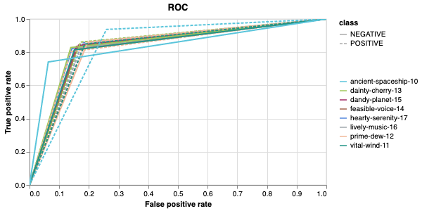
The cross-validation runs are uploaded to the wandb dashboard along with various interactive custom charts and tables which we provide as part of our pipeline. These are conceptually identical to those generated by sweep or train. A small subset of plots are provided for reference. Interactive versions of these and more plots are available on wandb.

Here is an example of a full wandb generated report:

You may inspect your own generated reports after they complete.

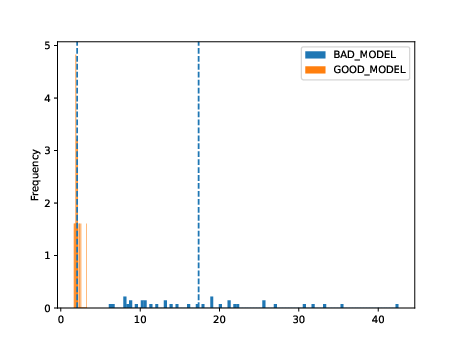
10. Compare different models

The aim of this step is to compare performance of different deep learning models efficiently while avoiding computationally expensive re-training and data download in conventional model comparison. In the case of patient data, they are often inaccessible for privacy reasons, and in other cases they are not uploaded by the authors of the experiment.

For the purposes of this simple case study, we compare multiple sweeps of the same dataset as a demonstration. In a real life application, existing biological models can be compared against the user-generated one.

fit_powerlaw \
  ../results/sweep_out/model_files \
  -o ../results/fit
# -m MODEL_PATH, path to trained model directory
# -o OUTPUT_DIR, path to output metrics directory

This tool outputs a variety of plots in the specified directory.

ls ../results/fit
# alpha_hist.pdf  alpha_plot.pdf  model_files/

Very broadly, the overlaid bar plots allow the user to compare the performance of different models on the same scale. A narrow band around 2-5 with few outliers is in general cases an indicator of good model performance. This is a general guideline and will differ depending on context! For a detailed explanation of these plots, please refer to the original publication.

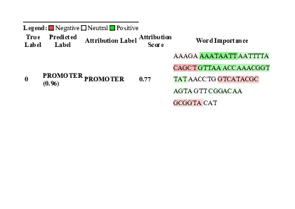
11. Obtain model interpretability scores

Model interpretability is often used for debugging purposes, by allowing the user to “see” (to an extent) what a model is focusing on. In this case, the tokens which contribute to a certain classification are highlighted. The green colour indicates a classification towards the target category, while the red colour indicates a classification away from the target category. Colour intensity indicates the classification score.

In some scenarios, we can exploit this property by identifying regulatory regions or motifs in DNA sequences, or discovering amino acid residues in protein structure critical to its function, leading to a deeper understanding of the underlying biological system.

gzip -cd ../data/promoter.fasta.gz | \
  head -n10 > ../data/subset.fasta
interpret \
  ../results/sweep_out/model_files \
  ../data/subset.fasta \
  -l PROMOTER NON-PROMOTER \
  -o ../results/model_interpret
# -t TOKENISER_PATH, path to tokeniser.json file to load data
# -o OUTPUT_DIR, specify path for output

ECK120010480 CSGDP1 REVERSE 1103344 SIGMA38.html
ECK120010489 OSMCP2 FORWARD 1556606 SIGMA38.html
ECK120010491 TOPAP1 FORWARD 1330980 SIGMA32 STRONG.html
ECK120010496 YJAZP  FORWARD 4189753 SIGMA32 STRONG.html
ECK120010498 YADVP2 REVERSE 156224  SIGMA38.html

Citation

Cite our manuscript here:

@article{chen2023genomicbert,
    title={genomicBERT and data-free deep-learning model evaluation},
    author={Chen, Tyrone and Tyagi, Navya and Chauhan, Sarthak and Peleg, Anton Y and Tyagi, Sonika},
    journal={bioRxiv},
    month={jun},
    pages={2023--05},
    year={2023},
    publisher={Cold Spring Harbor Laboratory},
    doi={10.1101/2023.05.31.542682},
    url={https://doi.org/10.1101/2023.05.31.542682}
}

Cite our software here:

@software{tyrone_chen_2023_8135591,
  author       = {Tyrone Chen and
                  Navya Tyagi and
                  Sarthak Chauhan and
                  Anton Y. Peleg and
                  Sonika Tyagi},
  title        = {{genomicBERT and data-free deep-learning model
                  evaluation}},
  month        = jul,
  year         = 2023,
  publisher    = {Zenodo},
  version      = {latest},
  doi          = {10.5281/zenodo.8135590},
  url          = {https://doi.org/10.5281/zenodo.8135590}
}